How to Measure the Spectral Linewidth of a Single-Frequency Laser?

In high-precision optical fields such as distributed acoustic sensing (DAS), coherent lidar, and quantum communication, the spectral linewidth of the laser is a key indicator determining performance. A narrower linewidth indicates higher coherence and lower phase noise, and it also enables a better signal-to-noise ratio in long-distance transmission.

However, as advanced lasers are now capable of generating single-frequency light at frequencies of kilohertz (kHz) or even sub-kilohertz levels, the challenge of accurately measuring such ultra-narrow linewidths has become a problem for engineers – because the resolution of standard testing instruments is already insufficient.

Therefore, this guide will delve deeply into the industry-standard Delayed Self-Heterodyne (DSH) method and provide a detailed analysis of the key optical devices and core components required for achieving precise measurements.

The Challenge with Standard Optical Spectrum Analyzers

The resolution bandwidth of a high-end grating-based optical spectrometer (OSA) is typically between 0.01 nm and 0.05 nm. At a wavelength of 1550 nm, a resolution of 0.01 nm is converted to the frequency domain and is approximately 1.25 GHz.

However, the actual linewidth of high-performance ultra-narrow-linewidth single-frequency fiber lasers is often only 1 kHz. For such a level of light source, an instrument with a 1.25 GHz resolution simply cannot capture the true spectral profile. The “wide peak” measured by it is actually just the response function of the instrument, reflecting the performance limit of the OSA rather than any defect of the laser itself.

Therefore, in order to accurately measure the linewidth at the kilohertz (kHz) level, we must shift the measurement dimension from the optical frequency domain of hundreds of terahertz to the radio frequency domain of MHz. Only in this way can high-resolution electrical spectrum analyzers (ESA) be of any use.

The Solution: Delayed Self-Heterodyne (DSH) Method

The core of the Delayed Homodyne (DSH) technology is to convert the difficult-to-measure optical phase noise into an easily detectable intensity noise through electronic means. Compared to the traditional dual-laser comparison method (which relies on expensive and difficult-to-stabilize ultra-stable reference lasers), DSH ingeniously allows the laser to interfere with its own delayed version.

In terms of specific implementation, the laser to be tested is split into two by the optical fiber coupler:

• Delay line: The light beam passes through a long single-mode optical fiber or an optical delay line. As long as the delay time is much longer than the coherence time of the laser, the output light will be completely incoherent from the other path, thus effectively equivalent to an independent reference source.
• Frequency shifting path: The light beam undergoes frequency shifting through an acousto-optic modulator (AOM), introducing a precise radio frequency offset (typically ranging from 40 MHz to 200 MHz).

Finally, the two beams of light converge at the second coupler to generate a beat frequency. The high-speed photodetector converts the beat frequency signal into an electrical signal and sends it to the electro-spectrum analyzer (ESA) for analysis. Since the center frequency has been shifted by the AOM, the laser line will be perfectly centered on the corresponding RF frequency on the ESA screen, thus completely avoiding the interference of low-frequency flicker noise and DC signals.

Critical Components of a DSH Measurement Setup

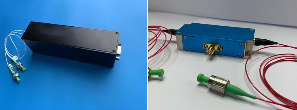
To build a high-precision DSH system, it is essential to select high-quality optical components to strictly control phase noise, signal degradation and insertion loss.

Delayed optical fiber (fiber span)

The length of the delay line is crucial. To ensure that the two beams of light are completely decoupled (unrelated), the optical delay must be much longer than the coherence time of the laser (typically requiring more than 6 times). For example, for a 1 kHz narrow linewidth laser, its coherence length can reach several tens of kilometers. This requires the use of precise fiber spools or adjustable delay lines to precisely control the optical path difference and minimize the introduction of polarization mismatch and high attenuation.

Optical fiber coupled acoustic-optic modulator (AOM)

If an AOM is not introduced, the two arms of the light beam will directly undergo direct frequency modulation (at 0 Hz), resulting in the laser’s true waveform being submerged in the strong background noise of the photodetector. By using a high-performance AOM, stable and pure frequency shifts (such as 80 MHz or 150 MHz) and high carrier extinction ratio can be provided, thereby perfectly preserving the inherent waveform of the single-frequency light source.

Photoelectric detector and electro-spectrum analyzer (ESA)

The high-speed photoelectric detector is responsible for converting the combined optical signal into a radio frequency signal. Its bandwidth must cover the modulation frequency of the AOM. Finally, the electro-spectrum analyzer (ESA) captures and displays the power spectrum of the beat frequency signal, which is used for subsequent linewidth assessment.

How to Calculate the Linewidth from the ESA Spectrum

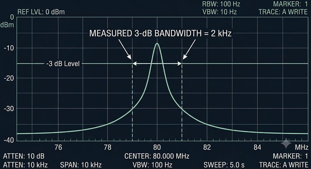
Once the beat note is displayed on the Electrical Spectrum Analyzer, you will observe a characteristic symmetric profile centered at the AOM modulation frequency.

Identify the Profile Shape: If the laser phase noise is dominated by white noise, the resulting RF spectrum will exhibit a Lorentzian lineshape. If environmental flicker noise or thermal fluctuations dominate, it may resemble a Gaussian lineshape or a Voigt profile (a combination of both).

The Calculation for Lorentzian Profiles: For a pure Lorentzian lineshape, the full-width at half-maximum (FWHM) of the RF beat note measured at the 3-dB points on the ESA is exactly twice the actual optical linewidth of the laser.

Formula: Laser Linewidth = (Measured 3-dB Bandwidth) / 2

Therefore, if your ESA measures a 3-dB bandwidth of 2 kHz at the 80 MHz peak, your single-frequency laser has a true spectral linewidth of 1 kHz.

The Calculation for Gaussian Profiles: If the profile is predominantly Gaussian due to external vibrations, the true laser linewidth is calculated by dividing the 3-dB bandwidth by the square root of 2 (approximately 1.414).

To Conclude

For accurate measurement of the spectral linewidth of a single-frequency laser, it is normally required to move away from the conventional optical techniques to the radio frequency heterodyne technique. With the help of the technique of delayed heterodyne, along with the use of ultra-narrow linewidth single-frequency light sources, special fiber-coupled AOMs, and delay lines, one can accurately characterize the linewidth performance up to the sub-kHz range.

Whether you are concerned with advanced laser radar applications or with optical fiber sensing technologies, our technical experts are available to offer customized optical testing solutions for your needs. You can freely contact us to know more about our integrated range of products, including ultra-narrow linewidth single-frequency fiber lasers, reliable fiber-coupled AOMs, and customized optical delay lines.